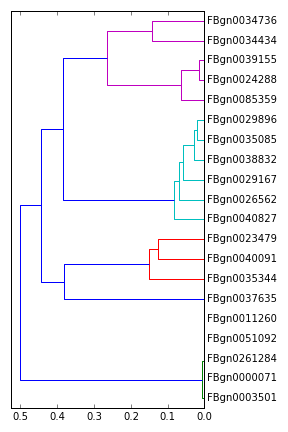
Gene- and sample-wise hierarchical clustering

A straight-forward approach to hierarchical clustering is computing a distance matrix from the appropriately transformed data matrix, which can then be used as input to hierarchical clustering routines. DGEclust aids this type of analysis by providing a way of computing such a distance matrix based on the output of the Gibbs sampler. Let's compute the distance matrix of the top 20 differentially expressed genes, as these were identified in the previous section:

1 from dgeclust import compute_similarity_vector
2 
3 idxs = np.argsort(res.FDR)[:20]                      # identifies the top 20 DE genes
4 simvec, nsamples = compute_similarity_vector(mdl, inc=idxs, compare_genes=True)

The above statement computes the condensed similarity matrix (represented as a vector) of the top 20 differentially expressed genes in the passila dataset. If the inc argument is omitted, then all genes are considered (this should be avoided for computational reasons!). The default value of the compare_genes argument is False, in which case the similarity vector between groups of samples is computed, instead. As in the case of the compare_groups function, compute_similarity_vector provides arguments for controlling which samples should be post-processed (t0, tend and dt) and the number of cores to be used (nthreads). Default values are the same as for the compare_groups function. In particular, a burn-in period of 5K iterations is assumed (t0=5000).

Having computed the similarity vector, we can proceed as follows:

1 import scipy.cluster.hierarchy as hr
2 
3 pl.figure(figsize=(4,6))
4 hr.dendrogram(hr.linkage(1-simvec), labels=res.FDR[idxs].index, orientation='right');