Processing the data

Next, we need to process the data using DGEclust. At the IPython terminal, type the following:

1 from dgeclust import CountData, SimulationManager
2 from dgeclust.models import NBinomModel
3 
4 mgr = SimulationManager()
5 
6 data = CountData(counts_filt, groups=['treated', 'treated', 'treated', 'untreated', 'untreated', 'untreated', 'untreated'])
7 mdl = NBinomModel(data, outdir='sim_output')
8 
9 mgr.new(data, mdl)

DGEclust is distributed as the python package dgeclust, which you can import and use at the IPython command prompt. At line 4 above, we create a new SimulationManager object, which we will use for initiating simulations.

At line 6, we create a CountData object, which takes as input the filtered count data and a list of strings representing the group assigment (i.e. treated or untreated) of each sample. If group is omitted, each sample is assumed to be a group on its own. This is a very simple way to indicate the presence or absence of biological replicates. The CountData constructor also accepts a lib_sizes argument, which is a list of normalisation factors, one for each sample. If omitted, as above, these normalisation factors are computed automatically using the same method DESeq uses.

At line 7, we create an NBinomModel object, which models the data using a Negative Binomial distribution. Simulation results are saved in the directory specified by the argument outdir (sim_output in this case). If this argument is omitted, the default destination is the sub-directory _clust in the current directory.

Finally, at line 9, we fire up a simulation using the new method of the mgr object and the data and model objects we created earlier as arguments. Notice that the new method returns immediately at the command prompt. This permits running additional simulations (i.e. by creating new CountData and NBinomModel objects and calling new with these as arguments) and inspecting them while they are running, as we shall see below. If this behavior is undesirable, we can modify it using the bg=False argument. The above command runs a Gibbs sampler for a default of 10K iterations. A different simulation length can be specified using the argument niters. By default, the data are processed in parallel using all available processing cores in the system. Again, this behaviour can be modified using the nthreads argument.

Depending on the size of your data and system resources, the above simulation will take several minutes to finish. Its progress can be checked periodically by calling the plot_progress method of the mdl object:

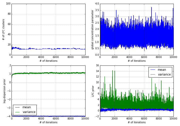
1 mdl.plot_progress(fig=pl.figure(figsize=(10,7)))

After the end of the simulation, the output of the above statement looks as follows:

Thanks to the blocked Gibbs sampler DGEclust uses internally, the algorithm converges rapidly, after ~1000 iterations. DGEclust uses a Hierarchical Dirichlet Process (HDP) mixture model to cluster the log-fold changes (LFCs) across genes and across groups of samples. The top left plot illustrates that an average of around 12 clusters are supported by the data. The top right plot illustrates the trace of the global concentration parameter of the HDP. In addition, DGEclust assumes normal priors for the log-dispersion parameter of the Negative Binomial distribution and for the LFCs. The bottom panels illustrate the traces of the estimated mean and variance for each of these two priors.

Before attempting any further analysis, it is important that the traces illustrated in the abiove figure reach a steady state. This means that we might need to extend the simulation beyond just 10K iteration. This can be achieved by loading the state of a previously saved simulation and using this as the initial state for a new simulation, as shown below:

1 mdl = NBinomModel.load('sim_output')
2 mgr.new(data, mdl, niters=5000)

The above code will extend the simulation previously stored in sim_output for another 5K iterations.

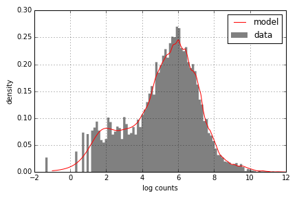
At any point during the simulation, we can check how well the model fits the data using the plot_fitted_model method of an NBinomModel object. For example, for the treated1fb sample, we have:

1 mdl.plot_fitted_model('treated1fb', data);

Obviously, a similar plot can be constructed for each sample in the data.

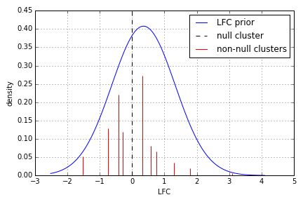
In addition, we can inspect the estimated LFC clusters, using the plot_clusters method of the NBinomModel object:

The null-cluster corresponds to no differential expression, while negative (positive) LFC clusters imply under(over)-expression in relation to the null cluster.

The next step is to post-process these results in order to test for differential expression. Learn how!